Credit Score Prediction With Scorecards Method
I. Introduction and Background
PinjamPintar is a financial institution with a deep commitment to financial services. PinjamPintar is dedicated to meeting financial needs or providing lending services to individuals seeking personal financing. Like other financial institutions, PinjamPintar also faces challenges in the lending decision-making process. This process involves manual assessments that are time-consuming and at risk of subjective bias. Not only that, the risk associated with a Non-Performing Loan (NPL) or unpaid debt is always a major concern for PinjamPintar. These problems encourage PinjamPintar to find solutions that can improve efficiency and accuracy in making loan decisions. One approach that can be taken is the use of credit scores or credit score prediction models.
Credit scoring is a method of evaluating the credit risk of loan applications. Using historical data and statistical techniques, credit scoring tries to isolate the effects of various applicant characteristics on delinquencies and defaults. The method produces a “score” that a bank can use to rank its loan applicants or borrowers in terms of risk. To build a scoring model, or “scorecard,” developers analyze historical data on the performance of previously made loans to determine which borrower characteristics are useful in predicting whether the loan performed well. A well-designed model should give a higher percentage of high scores to borrowers whose loans will perform well and a higher percentage of low scores to borrowers whose loans won’t perform well. But no model is perfect, and some bad accounts will receive higher scores than some good accounts (Loretta J. Mester, 1997).
Credit scoring has some obvious benefits that have led to its increasing use in loan evaluation. First, scoring greatly reduces the time needed in the loan approval process. A study by the Business Banking Board found that the traditional loan approval process averages about 12–1/2 hours per small-business loan, and in the past, lenders have taken up to two weeks to process a loan (Allen). Credit scoring can reduce this time to well under an hour, although the time savings will vary depending on whether the bank adheres strictly to the credit score cutoff or whether it reevaluates applications with scores near the cutoff. Another benefit of credit scoring is improved objectivity in the loan approval process. This objectivity helps lenders ensure they are applying the same underwriting criteria to all borrowers regardless of race, gender, or other factors prohibited by law from being used in credit decisions (Loretta J. Mester, 1997).
Limitations of credit scoring, the accuracy of the scoring systems for underrepresented groups is still an open question. Accuracy is a very important consideration in using credit scoring. Even if the lender can lower its costs of evaluating loan applications by using scoring, if the models are not accurate, these cost savings would be eaten away by poorly performing loans. The accuracy of a credit scoring system will depend on the care with which it is developed. The data on which the system is based needs to be a rich sample of both well-performing and poorly-performing loans. The data should be up to date, and the models should be re-estimated frequently to ensure that changes in the relationships between potential factors and loan performance are captured (Loretta J. Mester, 1997).
There are several development objectives of credit score prediction for PinjamPintar, namely:
- Build a technology-based application that automatically assesses loan applicants based on various factors, including credit history, income, employment, marital status, and other relevant variables.
- Identify applicants who have a high risk of defaulting on their loans, which can help reduce the risk of Non Performing Loan (NPL).
- Improve efficiency and consistency in assessing credit risk by using predictive models based on historical data and trained algorithms that enable more objective and consistent decision making.
- Transforming PinjamPintar’s decision-making process from manual lending to more efficient and effective use of credit scores or credit score prediction models.
In building the PinjamPintar scorecard, the logistic regression method is used. Logistic regression is a statistical model that is well suited for modeling binary or categorical outcomes. The goal of an analysis using logistic regression is the same as that of any model-building technique used in statistics — to find the best fitting and most parsimonious, yet reasonable model to describe a relationship between a dependent and one or more independent variables. Logistic regression produces models that are easy to explain and implement and has been widely accepted in the banking industry as the method of choice (Christine Bolton, 2009).
II. Dataset Description
The dataset comes from loan_default. This dataset has 255,347 accounts (assumption) from 18 variables, but only uses a few variables that are relevant in influencing/evaluating loan default. The data is a collection of information that includes demographic, financial, and loan. The data consists of :
· 15 predictors/potential characteristic
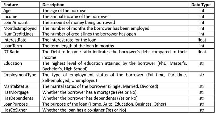
· 1 response/target variable

III. Scorecard Development
Developing scorecards is one of the important steps in credit risk assessment. Before entering the stage of developing scorecards, it is important to understand that scorecards are statistical tools that assist in making decisions based on historical data and applicant characteristics. Scorecards are used to assess the credit risk of customers or loan applicants in making decisions regarding loan approval or rejection, minimizing losses due to unpaid loans, and optimizing credit decisions.
In its simplest form, a scorecard consists of a group of characteristics, statistically determined to be predictive in separating good and bad accounts. Scorecard characteristics may be selected from any of the sources of data available to the lender at the time of the application. Examples of such characteristics are demographics (e.g., age, time at residence, time at job, postal code), existing relationship (e.g., time at bank, number of products, payment performance, previous claims), credit bureau (e.g., inquiries, trades, delinquency, public records), real estate data, and so forth (Naeem Siddiqi, 2006).
Each attribute (“Age” is a characteristic and “23–25” is an attribute) is assigned points based on statistical analyses, taking into consideration various factors such as the predictive strength of the characteristics, correlation between characteristics, and operational factors. The total score of an applicant is the sum of the scores for each attribute present in the scorecard for that applicant (Naeem Siddiqi, 2006).
The steps for developing scorecards are:
1. Explore Data
The data exploration stage is carried out to understand and analyze the data that will be used in model development. At this stage, simple statistics such as value distribution, mean/median, and checking the integrity of each data are carried out. The following is data exploration of each predictor:
· Predictor Age

In the figure above it can be concluded that:
- The youngest debtor is 18 years old.
- Three-quarters of the debtors are up to 56 years old. The rest are over 56 years old.
- The oldest debtor is 69 years old.
- There are differences in age between the two groups. The age of borrowers in default 0 has a higher mean and greater variation compared to default 1.
· Predictor Income

In the figure above it can be concluded that a borrower who defaults has a slightly lower average income than a borrower who does not default.
· Predictor Loan Amount

In the figure above it can be concluded that borrowers who default have a higher average loan amount than borrowers who do not default.
· Predictor Months Employed

In the figure above it can be concluded that:
- The number of months employed for both defaulted and non-defaulted borrowers has a minimum value of 0 months and a maximum of 119 months.
- Data integrity is performed where there are no data inconsistencies such as months employed data exceeding the borrower’s age.
- In the non-defaulted group (default 0), the average number of months employed (months employed) is longer than the defaulted group (default 1).
· Predictor Number Credit Lines

In the figure above it can be concluded that:
- The average number of credit lines (number credit lines) is almost the same for both groups. The non-defaulted group (default 0) has an average of about 2.49 credit lines, while the defaulted group
(default 1) has an average of about 2.59 credit lines. - Most individuals in both groups have 1, 2, 3, or 4 lines of credit.
- There is no significant difference in the average number of credit lines between the two groups.
· Predictor Interest Rate

In the figure above it can be concluded that:
- There is a significant difference in interest rates between the two groups. Higher interest rates may be an indication of higher credit risk.
- The average interest rate is higher in the defaulted group (default 1) compared to the non-defaulted group (default 0).
- Most individuals in both groups have interest rates between 11 and 21.37, but the default 1 group tends to have higher interest rates.
· Predictor Loan Term

In the figure above it can be concluded that:
- The average loan tenure (loan term) is almost the same between the two groups, both those who have defaulted (default 1) and those who have not (default 0).
- Most individuals in both groups have a loan tenure between 24 to 48 months.
- Loan tenure ranges from 12 to 60 months.
- There is no significant difference in loan tenure between the defaulted and non-defaulted groups.
· Predictor DTI Ratio

In the figure above it can be concluded that:
- The DTI ratio ranges from 0.1 to 0.9.
- The average debt-to-income ratio (DTI ratio) in the two groups, both those in default (default 1) and those without (default 0), are relatively close to each other. Although the average DTI ratio is slightly higher in the Default 1 group.
· Predictor Education
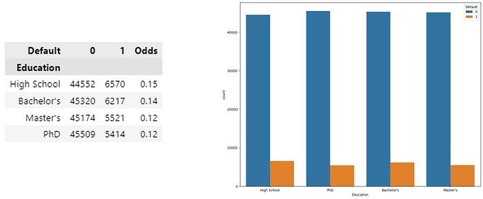
In the figure above it can be concluded that:
- Lending to individuals with higher education levels tends to have a lower default risk.
- The default ratio (Default 1) tends to be lower for individuals with higher education levels.
· Predictor Employment Type

In the figure above it can be concluded that:
- Unemployed individuals have the highest default odds, which is around 0.16. This indicates that people who are unemployed have a higher risk of default. This may be due to the lack of a stable source of income.
- Individuals who work part-time also have fairly high default odds, which are around 0.14. Although lower than those who are not employed, they still have a significant default risk.
- Meanwhile, self-employed and full-time individuals have lower default odds of around 0.13 and 0.10, respectively. This suggests that having a full-time job or self-employment status can reduce the risk of default.
· Predictor Marital Status
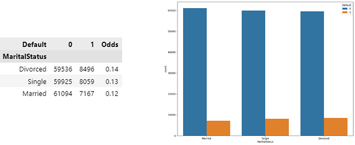
In the figure above it can be concluded that:
- Divorced individuals have the highest default odds. This suggests that divorced marital status may increase the risk of default.
- Unmarried individuals (single) have slightly lower default odds. Although lower than the divorced ones, the marital status “single” also still has a significant default risk.
- Meanwhile, individuals who are married (Married) have lower default odds of around 0.12. This suggests that “married” marital status may be associated with a lower default risk.
· Predictor Has Mortgage
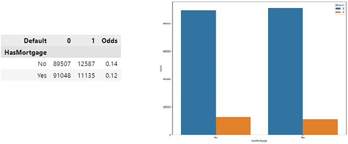
In the figure above it can be concluded that individuals who do not have a mortgage (no) have higher default odds of about 0.14. This suggests that not having a mortgage may increase the risk of default.
· Predictor Has Dependents
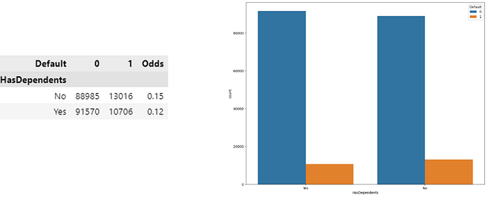
In the figure above it can be concluded that:
- Borrowers without dependents (has dependents: no) have a default rate of about 13%. This means that about 13% of borrowers without dependents defaulted in this dataset.
- Borrowers with dependents (has dependents: yes) have a similar default rate of around 12%. This means that about 12% of borrowers with dependents defaulted.
- Odds (the ratio of borrowers who default to those who do not) for these two groups are also relatively close to each other, with values of around 0.15 for borrowers without dependents and around 0.12 for borrowers with dependents.
· Predictor Loan Purpose
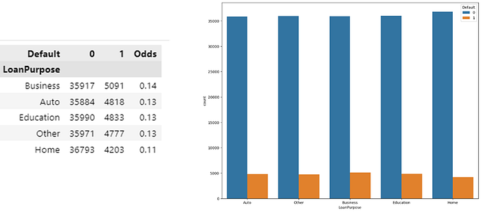
In the figure above it can be concluded that:
- “Business” purpose loans have a higher default rate than others.
- Loans with the purpose of “Auto,” “Education,” and “Other” have a default rate of around 13%, which is about the same.
- Loans with the purpose of “Home” have the lowest default rate, around 11%.
· Predictor Has Co-Signer

In the figure above it can be concluded that loans with co-signers have a lower default rate than loans without co-signers.
2. Handle Missing Values and Outliers
Of the 15 predictors/potential characteristics given, missing value checking will then be carried out. The results of the missing value check can be seen in the following figure:

From the figure above, it can be confirmed that there are no missing values in the data set. This indicates that the data is complete and there is no missing or unfilled information in the variables. In addition, there are no outliers in the dataset so at this stage the steps to handle missing values and outliers do not need to be done.
3. Check Correlation
The next step is to check the correlation on the numerical predictor. The results of checking the correlation can be seen in the figure below.
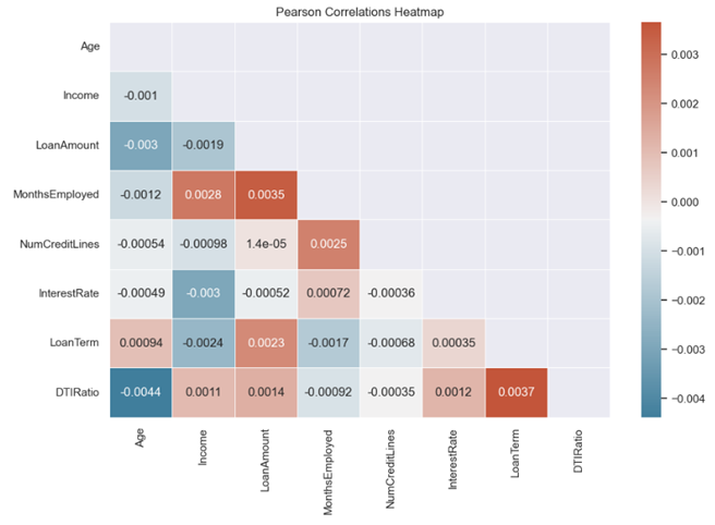
Based on the figure above, the correlation between variables is low. The largest positive correlation is found in the loan term predictor and the DTI ratio predictor of 0.0037. this indicates that when the value of one predictor increases, the value of the other predictors also tends to increase. Meanwhile, the largest negative correlation is found in the age predictor and the DTI Ratio predictor of -0.0044 which indicates that when the value of one predictor increases, the value of the other predictors tends to decrease and vice versa.
When checking the correlation, there is no multicollinearity in the numerical predictors. Multicollinearity is a condition where two or more predictors have a strong relationship with each other which causes the predictors to not be independent and have a significant level of correlation between each other.
4. Initial Characteristic Anaysis
At this stage, each characteristic/predictor is analyzed to predict the credit score or total point score of an applicant by binning the numerical predictors. Binning is the process of grouping or classifying numerical values into categories or “bins.” The number of binning is 5 categories. The purpose of the binning process on the numerical predictor is to make continuous data simpler and easier to interpret. The results of the binning process can be seen in the following image.
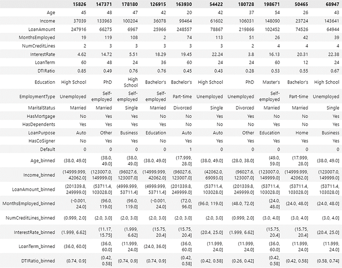
Next, a contingency table is made where the Contingency table functions to describe or present the relationship between two or more categorical variables. The results of each category can be seen in the following contingency table.

5. Statistical Measures
In the statistical measure, the WOE and IV values are found.
· Weight of Evidence (WOE)
WOE is used to measure the strength of each attribute in each category. WOE calculated as follows :

To better understand WOE, we would like to stress the following:
- %Bad is not equivalent %Bad Rate. % Bad is the percentage of bad accounts in a score band over all bad counts. Same understanding applies to %Good in the example.
- It does not matter whether %Good or %Bad should be chosen as the numerator. If the two measures exchange their positions in the division, the sign of WOE for each score band will reverse while the magnitude will remain unchanged. There is no impact on the subsequent calculation for IV.
- Multiplication by 100 is optional (Alec Zhixiao Lin, 2014).
The value of WOE can be seen in the following figure.

· Information Value (IV)
IV is used to measure the strength of each characteristic. The IV value is obtained from the sum of the contribution IV of each attribute. The following is how IV is calculated :

In such cases, we consider following rules of thumb suggested by Siddiqi for evaluating IV still applies to the binary dependent variable for the alternative IV:

The IV and strength values for each characteristic can be seen in the following table.

From the table above, the results show that there are 9 characteristics that have unpredictive strength, 3 characteristics that have weak strength and 3 characteristics that have medium strength. After that, check the independence test, where individually each characteristic has a relationship with the target variable (default/no default). The table of the independence test can be seen in the following figure.

6. Check Logical Trend and Business/Operational Considerations
At this stage, a manual check is carried out by the developer by making a WOE plot. Checking is done on each characteristic, namely:
· Characteristic 1 : Age

From the figure above, the higher the age of an applicant, the lower the risk of default, while the lower the age, the higher the risk of default. Generally, the younger a person is, the less credit experience they have and therefore the higher the risk of default. Conversely, the older a person is, the more credit experience they have that can demonstrate their credit quality, resulting in a lower risk of default.
· Characteristic 2 : Income

From the figure above, it can be seen that the more income the risk of default is low due to the greater ability of an applicant to repay the loan, while the lower the income, the higher the risk of default because someone may have difficulty repaying the loan.
· Characteristic 3 : Loan Amount

From the figure above, it can be seen that the lower the loan amount, the lower the risk of default, while the higher the loan amount, the higher the risk of default. This is because small loans are easier to repay than large loans that require higher monthly payments.
· Characteristic 4 : Months Employed

From the figure above, it can be seen that the fewer months employed, the higher the risk of default and the greater the months employed, the lower the risk of default. Generally, an applicant who has worked in the same job for a longer time tends to have better job stability. They are more likely to have a consistent income and can easily repay their loans
· Characteristic 5 : Number Credit Lines

From the figure above, the lower the number of credit lines, the lower the risk of default while the higher the number of credit lines, the higher the risk of default. This is because fewer credit lines may indicate that a person is financially responsible and can manage their debt well, hence lower default risk.
· Characteristic 6 : Interest rate

From the figure above, the lower the interest rate, the lower the risk of default while the higher the interest rate, the higher the risk of default. When interest rates are low, monthly installments are more affordable for an applicant. This makes them more likely to repay on time whereas when interest rates are high, monthly installments become more expensive and this can cause difficulties for borrowers in repaying their loans. This can increase the chances of late payment or default.
· Characteristic 7 : Loan Term

From the figure above, it can be seen that the smaller the loan term, the lower the default risk while a large loan term allows the default risk to be higher. With a short loan term, an applicant has to repay the loan in a short period of time. This means that monthly installments will be higher, but borrowers will pay off their loans faster. Due to the high monthly installments, applicants tend to have enough income to repay the loan on time, which reduces the risk of default. With a long loan term, the monthly installments are lower, but applicants have to repay the loan over a longer period of time. Despite lower monthly installments, a long loan term increases the risk of default as many changes in an applicant’s financial situation may occur over a long period of time.
· Characteristic 8 : DTI Ratio

From the figure above, it can be seen that the less the DTI ratio, the lower the risk of default but the greater the DTI Ratio, the higher the probability of default risk. If the DTI ratio of an applicant is low, it means that the applicant has more income available to pay the debt. In this context, the lower the DTI ratio, the lower the default risk because the applicant has a good financial capacity to repay the loan on time. Meanwhile, when the applicant’s DTI ratio is high, it means that the applicant has utilized most of its income to pay debts. In this situation, the higher the DTI ratio, the higher the default risk. Applicants with a high DTI ratio tend to have little financial flexibility, and small changes to their finances can result in difficulty paying the loan.
· Characteristic 9 : Education

From the figure above, it can be seen that high school education has the highest default risk while PhD education has the lowest default risk compared to bachelors and masters. An applicant with higher education tends to have a job with higher income, which can help in repaying the loan on time.
· Characteristic 10 : Employment Type

From the figure above, applicants with employment type, namely unemployed, have a high default risk while full-time employment type has the lowest default risk compared to part-time and self-employed. This is because applicants who work full-time (full-time) tend to have a more stable and high income Sufficient income can help someone to pay loans on time.
· Characteristic 11: Marital Status

From the figure above, marital status divorced has a higher default risk rate than married or single. Divorce can have financial repercussions, such as the division of assets and financial obligations that can affect a person’s ability to repay a loan.
· Characteristic 12 : Has Mortgage

From the figure above, it can be seen that those with mortgages have a lower default risk than those without mortgages.
· Characteristic 13 : Has Dependents
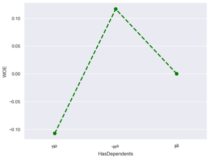
From the figure above, it can be seen that dependents make the risk of default lower than non-dependents. This is because applicants who have dependents such as children or other family members may be more responsible in managing their finances.
· Characteristic 14 : Loan Purpose

From the figure above, it can be seen that loan purpose home has a lower default risk than loan purpose auto, business, education and other.
· Characteristic 15 : Has Co-Signer

From the figure above, it can be seen that having a co-signer makes the risk of default lower than not having a co-signer. With a co-signer, the lender has two parties responsible for repaying the loan. If the primary borrower experiences financial difficulties, the co-signer can help repay the loan.
Based on the analysis of each characteristic, it can be concluded that all WOEs make business, logic and operational sense.
7. Design Scorecards
To create a scorecard design, a logistic regression model is used. To perform the modeling, not the original inputs of age, income, etc. (row input) to be used but the WOE of each attribute. Therefore, transform each data into WOE values for all predictors which can be seen in the following figure.

Next, do model selection using forward selection, this was chosen because there are many predictors so that the running time is not too long. Forward selection start with nothing, and add terms in order of significance (McNamara, 2016).
Furthermore, recall (sensitivity) is used as the main metric to select the best model. Recall is able to measure the extent to which the model correctly identifies borrowers who will actually default (true positives) from the overall borrowers who will actually default. The default rate in the sample is relatively high at (11%) indicating that many borrowers are likely to default, and the main goal is to reduce the default rate. Therefore maximize “rejection of bads” or maximize true positives to ensure that the model is effective in classifying borrowers who will actually default.
To select the best model, cross-validation with k-fold of 10 is used. In 10-fold cross-validation, the data is divided into 10 equal parts (folds). Then, the model is evaluated 10 times by taking each fold as test data one by one and the rest as training data. The evaluation results from each cross-validation iteration are used to measure the performance of the model, including recall.
This process helps ensure that the model’s performance is consistent and reduces the risk of overfitting. After going through 10-fold cross-validation, select the model with the highest recall value as the best model. The results of the recall score can be seen in the following figure.

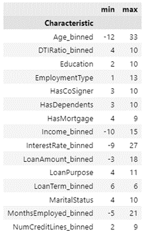
From the selection model, it is found that the best logistic regression model contains 1 predictor, namely Loan Purpose by 82%. Because there are very few predictors, if there is a slight change in the data, the prediction results are unstable. Based on these results, model adjustments were made, and the final scorecard consisted of 15 predictors. Next, the minimum points and maximum points for each characteristic were obtained. Then perform an evaluation on the training data which results in a recall of 68% and 69% on the testing data. The minimum and maximum points can be seen in the following figure.
8. Choose a Scorecard
In this stage, the development of a credit or risk model is used to assess the quality and performance of the prediction model. This involves selecting the final model or score that will be used to assess the credit or risk applicant. To select the most suitable model, a number of statistical metrics are used to measure its quality. The metrics used are AUC and KS Statistic. AUC is an evaluation metric used to measure the extent to which the model can distinguish between positive (1) and negative (0) classes. The AUC value can be seen in the following figure.

From the figure above, the AUC value in the train set is 0.74 which indicates that the model has a good ability to distinguish between positive and negative classes. While in the test set the AUC value is 0.75. The higher the AUC value (closer to 1), the better the model is at classifying.
Then check the KS Statistic (Kolmogorov-Smirnov Statistic), the KS Statistic measures the difference between two cumulative distribution functions, one for the positive class (1) and one for the negative class (0). the results of the KS statistic can be seen in the following picture.
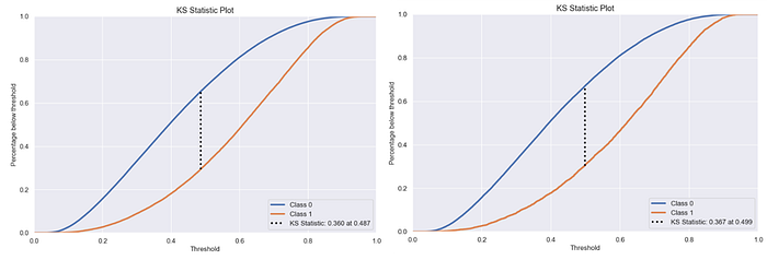
From the figure above, the KS Statistic reaches 0.360. At this point, it indicates that the model is good enough to distinguish between classes 0 and 1.
IV. Implementation Plan
In the implementation plan, setting the credit score cutoff (determining the credit score threshold) to obtain key decisions in the credit risk assessment process. The credit score threshold determines whether an applicant will be approved or rejected for a loan or credit. The selection of the cutoff score value of 150 is based on several considerations, namely based on the availability of data and score models that support the threshold. In addition, the cutoff selection is also based on the expected bad rate. This means that PinjamPintar estimates that applicants with scores below 150 have a higher or worse risk of default. So it is necessary to control credit risk by minimizing the approval of applicants with low credit scores.
The workflow of the credit process begins with inputting the applicant’s name, then inputting demographic, financial and loan data from the applicant, after successfully inputting the data, the next stage is modeling of credit scoring which will produce a credit score from an applicant. If an applicant has a score of more than 150 then the applicant will be approved, while if the applicant’s score does not exceed 150 but the value they have is more than 135 then the applicant will be reviewed again with several additional conditions. If these conditions are accepted by the applicant then the applicant will be approved otherwise the applicant will be declined. Then if the applicant’s score is less than 135 then the applicant will automatically be declined. For an overview of the workflow credit process, see the following image.

The results of the credit score prediction application overview can be seen in the following figure:

V. Conclusion and Recommendation
The logistic regression model that has been adjusted by selecting the right cut-off score is able to predict the credit score well. The model was able to distinguish between good and bad applicants with a recall rate of 68%. The overall quality of the model was rated as good with an AUC of 0.74. This indicates that the model can be used to support credit decisions well.
Based on the results of the analysis, there are several recommendations:
- For risk managers: utilize credit scoring models to assess applicants’ credit risk and make informed decisions on whether to approve or reject loans.
- For operations team: automate the decision-making process to improve efficiency and reduce manual review of applicants.
- For marketing teams: leverage models to target specific customer segments more effectively and develop focused marketing campaigns to acquire customers with lower default risk.
- For the next project recommendation is to try using other models such as decision tree, SVM or KNN to compare their performance in predicting credit scores.
VI. Reference
Alec Zhixiao Lin, PayPal Credit, Timonium, MD. 2014. Expanding the Use of Weight of Evidence and Information Value to Continuous Dependent Variables for Variable Reduction and Scorecard Development. Dept. of Mathematics & Statistics, Univ of Maryland, Baltimore, MD.
Christine Bolton. 2009. Logistic regression and its application in credit scoring. University of Pretoria.
Loretta J. Mester. 1997. What Is The Point Of Credit Scoring? Business review (Federal Reserve Bank of Philadelphia).
McNamara. 2016. SDS/MTH 291: Lecture Notes.
Naeem Siddiqi. 2006. Credit Risk Scorecards Developing and Implementing Intelligent Credit Scoring.
